Marrying Reinforcement Learning with Agentic Reasoning to accelerate Physical Design (PD)
Traditional chip development is sharply divided into two domains: the frontend (system specification and RTL/VHDL coding) and the backend (translating that programmatic description into transistor-level GDSII data via Electronic Design Automation (EDA) tools).
Currently, only 40% of a chip's development lifecycle is spent on frontend code. With the rise of agentic coding tools like Cursor and GitHub Copilot, frontend generation is accelerating massively. However, the backend physical design (PD) remains a severely manual bottleneck, consuming nearly 60% of design time with minimal AI support. Traditional PD takes 3 to 5 months to complete.
This creates a massive organizational throughput blockage. As frontend engineers generate designs faster, the backend cannot keep up, resulting in quantifiable costs in engineering payroll, reliance on outsourced design services, and lost market opportunities.
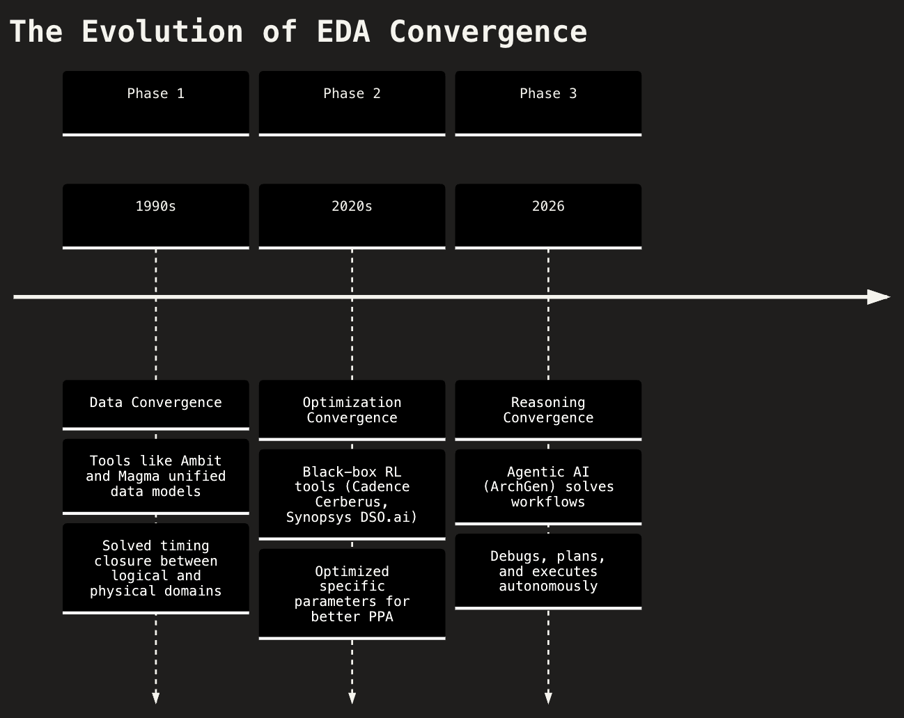
The Evolution of EDA Convergence
Magma built the engine that fixed the physics of timing closure; ArchGen AI is building the driver that fixes the economics of it. The EDA industry is progressing through three distinct phases of convergence:
- Phase 1 (Data Convergence): Mathematical determinism and unified data models solved timing closure between logical and physical domains.
- Phase 2 (Optimization Convergence): Black-box AI optimized specific parameters for better Power, Performance, and Area (PPA).
- Phase 3 (Reasoning Convergence): ArchGen AI enables autonomous reasoning through a combination of Reinforcement Learning (RL) and long-running Large Language Model (LLM) agents.
PD Code Architecture: RL + Agentic LLM
ArchGen achieves Reasoning Convergence by marrying a brute-force RL optimization engine with a high-level cognitive LLM brain.
The Reinforcement Learning (RL) Engine
We look at macro placement as a sequential game which is modelled in the following manner:
- The State: The chip die is discretized into a coarse grid. An edge-based Graph Neural Network (GNN) encodes the current state of the board, tracking the locations of already-placed macros and the dense web of netlist connectivity between them.
- The Action: The RL agent places exactly one macro at a time onto the grid. This turns floorplanning into a long-horizon decision process, meaning early placements irreversibly constrain the available space for later macros.
- The Reward: Intermediate rewards during placement are zero. Only after all macros are placed—and standard cells are temporarily assigned via a force-directed method—does the environment calculate a score. This reward is a mathematical linear combination of proxy metrics: Half-Perimeter Wirelength (HPWL), routing congestion, and density.
- The Algorithm: The model is trained using Proximal Policy Optimization (PPO) to navigate this massive state space and maximize that final reward score.
The Long-Running Agent (The LLM Brain)
While RL is a brilliant optimization engine, it is fundamentally a black box. Left to its own devices, an RL agent will often pack macros entirely too tightly to artificially minimize HPWL, creating massive routing congestion that makes timing closure impossible in a real backend flow.
The long-running LLM agent acts as the orchestrator that governs the RL tool, adding context, memory, and physical constraints to the process.
- Long-Term Memory Retrieval: Traditional EDA workflows suffer from amnesia. A long-running agent utilizes a database (like Supabase) to query historical run data. Before starting, it checks past iterations to see if, for example, a high utilization target previously caused catastrophic congestion in the Northeast quadrant of the die.
- Hyperparameter Planning: The Planner Agent reasons through the physics of the goal. If the user requests an aggressive 2.0 GHz target frequency, the LLM will adjust the RL environment's constraints before it runs—intentionally lowering the target placement density and widening the macro halos to give the router more breathing room.
- The Observer Loop: Once the RL model spits out a placement JSON, the LLM takes over. It pushes the coordinates into a full deterministic backend flow (like OpenROAD). The Analyzer Agent then reads the actual, physical ground-truth reports: Worst Negative Slack (WNS), Total Power, and Design Rule Check (DRC) violations, rather than relying on the RL's theoretical proxy reward.
- Deterministic Legalization: RL models are notorious for producing overlapping macros because they optimize for density grids, not discrete boundaries. To fix this, the agent orchestrates a strict 3-phase legalization fallback—Greedy Push → Random Search → Grid Snap—to guarantee a 100% physically valid, zero-overlap floorplan before initiating Clock Tree Synthesis (CTS).
By using the LLM to dynamically tune the RL reward weights, evaluate the physical outputs, and enforce deterministic legalizations, you eliminate the human iteration loop and achieve true autonomous workflow.
The PD Code Workflow: Step-by-Step
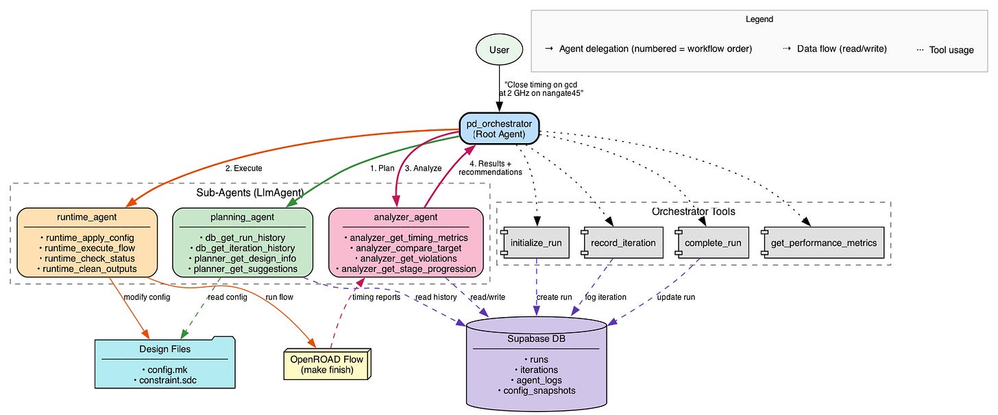
The system acts as a "Digital Senior Engineer" by breaking the massive physical design problem into distinct, manageable cognitive steps handled by specialized sub-agents.
Step 0: Initialization (Root Agent)
The human engineer provides a high-level natural language prompt (e.g.,
"Close timing on gcd at 2 GHz on nangate45"). The pd_orchestrator acts as the
lead manager. It immediately uses Orchestrator Tools (initialize_run) to create a new session
in the Supabase DB.
Step 1: The Planning Phase (planning_agent)
Before any code is executed, the orchestrator delegates to the Planning Agent. It reads the current target
specifications from the Design Files (config.mk, constraint.sdc). It queries the
Supabase DB (db_get_run_history) to look at past iterations. If it sees that a previous run
failed due to routing congestion, it factors that into its new strategy. Output: a concrete parameter
strategy to hit the 2 GHz target.
Step 2: The Execution Phase (runtime_agent)
Once a plan is formulated, the orchestrator hands it off to the Runtime Agent. It physically modifies the
parameters in the Design Files (runtime_apply_config). It triggers the actual EDA compiler via
the OpenROAD Flow (runtime_execute_flow) and monitors its progress
(runtime_check_status).
Step 3: The Analysis Phase (analyzer_agent)
After the OpenROAD flow finishes (or fails), the orchestrator brings in the Analyzer Agent to interpret the
raw results. It extracts WNS, TNS, power, and DRC metrics directly from the OpenROAD timing reports
(analyzer_get_timing_metrics). It figures out why the design failed or succeeded
(analyzer_get_violations) and writes its reasoning logs back to the Supabase DB.
Step 4: Results & Iteration
The pd_orchestrator takes the Analyzer's findings, uses Orchestrator Tools to log the completed
iteration (record_iteration), and returns the final results and recommendations to the user. If
the goal wasn't met, this loop repeats, utilizing the newly logged data to make a smarter plan for the next
iteration.
Benchmark Case Studies
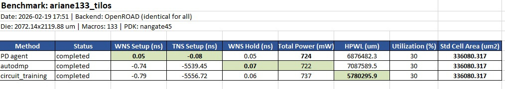
Ariane RISC-V CPU (133 Macros)
The Ariane RISC-V CPU benchmark exposes the fundamental flaw in pure reinforcement learning (RL) and analytical placers: they over-optimize for proxy metrics at the expense of routability and timing.
The Result: PD agent virtually closed timing with a WNS of 0.05ns and a
negligible TNS of -0.08ns. Meanwhile, both circuit_training and
autodmp failed catastrophically, hemorrhaging over -5500ns of Total Negative
Slack.
The Narrative: AlphaChip (circuit_training) achieved a visibly lower
Half-Perimeter Wirelength (HPWL of ~5.78M vs PD Agent's ~6.87M). However, because RL agents blindly pack
macros together to minimize wirelength, they create massive routing congestion that makes timing closure
impossible in the actual backend flow. PD Code's reasoning loop understands that relaxing HPWL slightly
gives the router breathing room, leading to a manufacturable design.
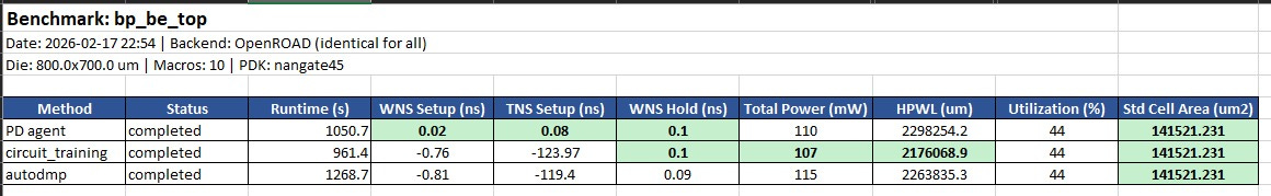
BlackParrot Backend (bp_be_top)
This mid-sized design (10 macros) reinforces the system's ability to navigate tradeoffs on highly constrained dies. Closing a massive Worst Negative Slack (WNS) violation typically requires a severe penalty in power or area.
The Result: PD agent is the only method that achieved positive setup slack
(0.02ns). The Google and AutoDMP baselines failed timing significantly (WNS ~-0.8ns).
The Narrative: Even on smaller designs where the die isn't heavily constrained, black-box optimization struggles to cross the finish line. PD Code successfully navigated the tradeoffs to produce a tapeout-ready macro placement while the established baselines required further human intervention.
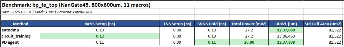
BlackParrot Frontend (bp_fe_top)
This benchmark shows what happens when the design is relaxed enough that all algorithms successfully close timing.
The Result: All three methods met timing constraints (WNS > 0). However, PD agent
delivered the lowest total power (26.00 mW) compared to the 27.2 mW generated by the
baselines, while tying autodmp for the best HPWL.
The Narrative: When timing isn't the primary bottleneck, PD Code dynamically shifts its optimization strategy to squeeze out significant power savings (a ~4.4% reduction) without sacrificing area or wirelength.
PD Code was deployed to optimize the backend of the Black Parrot RISC-V Processor:
- Timing: Fixed entirely. Total Negative Slack (TNS) was reduced from -28,646 ns to 0.
- Power: Decreased by 14.8%, dropping from 75mW to 64mW.
- Area: Achieved timing closure with only a marginal 3.8% increase in area.
ArchGen is building the Claude Code for physical design engineering. Through a simple terminal interface, a PD engineer provides a high-level description of their target, and our agentic system takes over—executing synthesis, floorplanning, placement, and routing in weeks rather than months.
If you love tinkering with chips, AI agents, and OpenClaw, or if you're like us and leave multiple Claude Code terminals running build workflows late into the night, we'd love to chat. Reach out to hari@archgen.tech or naveen@archgen.tech.
Disclaimer: This article was written with assistance from Gemini 3.1 pro and Claude Sonnet 4.5
Originally published on Substack.